Thank God for people like Ben Lambert.
I recently got acquainted with the BatchGetSymbols package, an auxiliary library to quantmod, and I am pretty impressed. It’s core function wraps a quality control protocol around quantmod’s getSymbols() function and returns a list with an execution summary and a daily price data datafame. This is a huge convenience improvement over the standard getSymbols() + lapply() batch query approach , which returns queries as individual xts objects.
Getting query returns as a few independent xts time series objects is fine when you’re only dealing with a couple fixed stocks; however, it’s incredibly cumbersome when you want to process a data on a large batch of stocks whose composition is conditional. BatchGetSymbols solves this issue by dumping query output into a single large dataframe that you can easily reshape into a list of matrices. I had some initial concerns that passing a large batch query would cause the Yahoo Finance API to kick the request back, but I am happy say that BatchGetSymbols impressed me. I was able to seamlessly pull years of price data for over 1000 stocks without any issues.

Being able to pull huge volumes of price data is invaluable in testing random ideas ~ for example, recently I became interested in pairs trading to see if artificial co-integrations could be created between stocks and peers with a high degree of co-movement. When ever pair trading strategies are discussed, the idea of co-integrated time series is presented with reference to two stocks derived from the same entity (e.g. GOOG & GOOGL). Being derived from the same entity, their prices should reflect the proportional claim on company equity and always generate the same returns in theory. However, for whatever reason, their trajectories can diverge for a short period of time and present an arbitrage opportunity where opposing long/short positions can be taken to generate profit – secure in the knowledge that the paths will re-converge in a short period of time due to fundamental forces.
The problem is that natural pairs are few and far between; However, I figured that given the sheer number of stocks in the market, there had many (if fleeting) co-integration opportunities. I wanted to do a large-scale scan of historic price data across large blocks of the market, find co-integration opportunities and then back-test them. This is where BatchGetSymbols becomes indispensable, because it allows you to pull tons without needing to implementing tons of your own quality controls.
- Is a requested stock only traded for only a portion of the date range?
– Don’t worry about it, it’ll be kicked out. - Did you miss-type a stock ticker?
– You’ll get a notification in the query return summary table. - Was the API only able to return a part of your query for some strange reason?
– Don’t worry, that will be flagged, as well. - etc.
Anyways, enough about data pulling process. Here is the theory: Co-integration opportunities can either be incidental (thousands of stocks, some are bound to move together for a short period of time by chance) or representative of real underlying similarities in risk-exposures between entities. There are a couple of basic controls that you can use to weed-out any price paths that aligned due to random chance: First, you can divide your stocks by market capitalization because implicit differences in liquidity, credit risk and information availability/quality. Then, you can use an extended formation period to further reduce the likelihood of find superfluous alignments.
I used a formation period of three (3) to (4) years and tested trades across mid and large cap stocks.
Here’s a quick tally breakdown of available stocks to search cross:
# > summary(stockInfo$CapGroup)
# ~ STOCK COUNT BY MCAP CLASS ~
# Small Mid Large Mega
# 3061 1063 682 22
# > tapply(stockInfo$MarketCap_num/1e9 %>% round(digits = 2), stockInfo$CapGroup, summary)
# ~ QUANTILES BY MCAP CLASS ($B) ~
# $Mid
# Min. 1st Qu. Median Mean 3rd Qu. Max.
# 2.000 2.710 3.920 4.521 5.920 9.970
#
# $Large
# Min. 1st Qu. Median Mean 3rd Qu. Max.
# 10.01 14.13 22.36 38.06 46.66 197.72
I used hierarchical clustering with average-linkages on daily returns data to establish equity groups with very similar price paths and high correlations. This resulted in stock groupings based on fundamental commonalities inherent to their specific sector. For example, regardless of the testing period, I would always see a cluster of 15-25 mid-sized regional US banks whose prices moved in tandem. This approach had the additional advantage of teasing out companies with abnormal returns due to idiosyncratic events, because their return-path deviations would be enough to kick them out of any clusters due to the low clustering cut-off point.
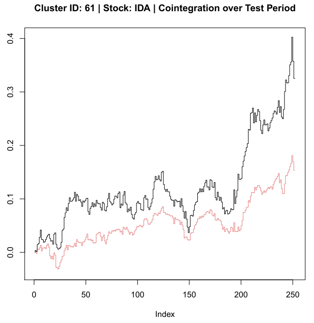
Typically, this approach would result in 5-10 clusters of stocks with 5 or more members with no cluster usually having more than 40 members. Once clusters were established, each member would be evaluated independently against the performance of it’s peers. Peer stocks would be packaged into an equally weighted cluster index, which reflected mean performance of the group and diversified out the impact of any minor company-specific events. Co-integration was evaluated using an augmented dickey-fuller test on stock-to-index linear regression residuals and accepted if the returned P-value was less than 5%. The trading strategy would the be back-tested against the formation period (offers no insights, but looks cool) and a short period of time right after it (typically 6 – 12 months).
The one thing I noticed about trying to execute this kind of strategy is that there timing and allocation factors that need to be balanced, whose challenges I am yet to resolve.
- Timing: If the co-integration holds during the forward testing period, divergences seem to result mainly from company-specific events and require at least a month to resolve themselves. This means that you might not see a re-convergence before the end of the testing period if divergence occurs fairly late. This pushes you to use longer periods; however the longer the testing period, the more likely co-integration relationship disappears.
- Allocation: Since cluster-indexes are held constant during the testing period, if one or a handful of members’ price paths significantly deviate from their peers, then it can destroy the co-integration relationship. If you start reshuffling clusters, then trade costs can quickly wipe away any gains.
To recap:
- 4 years of data for cluster formation. 6-12 months for testing.
- 1,000 stocks -> 5 – 10 clusters (appx. 150-200 stocks, total) -> 15 – 25 valid co-integrations.
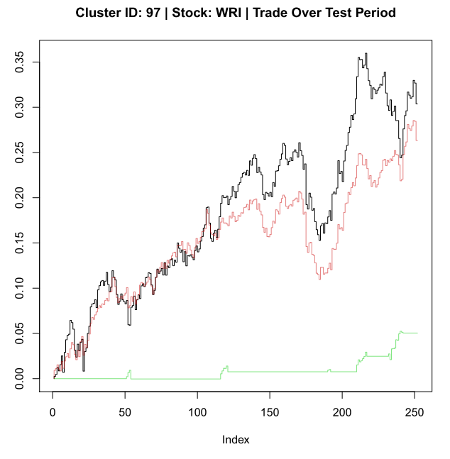
- Trade returns: visually, hit or miss. Need to program trade performance metrics.
- Fun concept to play around with, though. Probably works horribly in it’s current state when you factor in transaction costs.
A HIT
A MISS

If you’re interested in the subject of co-integration, here’s a list of great resource I found.
- Ben Lambert’s lectures on time series analysis: https://www.youtube.com/channel/UC3tFZR3eL1bDY8CqZDOQh-w
- Code walk-throughs that are much better than mine:
- https://analyticsprofile.com/algo-trading/pair-trading-part-2-code-correlation-based-pair-trading-strategy-in-r/
- https://www.quantstart.com/articles/Cointegrated-Time-Series-Analysis-for-Mean-Reversion-Trading-with-R
- https://www.quantstart.com/articles/Cointegrated-Augmented-Dickey-Fuller-Test-for-Pairs-Trading-Evaluation-in-R
Here’s the code. The parameters code-block provides plenty of controls you can play around with.
# Set-up Environment ——–
rm(list = ls()); invisible(gc())
if(dev.cur() > 1){dev.off()}
setwd(‘C:/Users/…’)
require(lubridate)
require(magrittr)
require(quantmod)
require(BatchGetSymbols)
require(MASS)
require(ggplot2)
require(purrr)
require(sparcl)
require(tseries)
‘%nin%’ = Negate(‘%in%’)
cat(“\014”) # Clear Console
# ~~~~~~~~~~~~~~~~~~~~~~~~~~~~~~~~~~~~~~~~~~~~~~~~~~~~~~~~~~~~~~~~~~~~~~~~~~~~~~~~~~~~~~~~~~~~~~~~~~~~~~~~~~~~~~~~~~~~~~~~~~~~~~~~
# Set Other Model Parameters —–
param.minClust = 5 # Mininum number of members per cluster
param.trainLength = 4 # Duration, years, over which to compile equity-clusters
param.seedDate = ‘2010-01-01’ # Starting date for training data … moved forward in test.length increments
param.testLength = 12 # Duration, months, over which to execute trade strategies
param.CapFocus = ‘Mid’ # Selects market-cap group for train/test execution.
# Values :: (Small, Mid, Large, Mega)
# Typically use Mid/Large, based on group size.
param.dfp = .05 # Dickey-fuller p-value cut-off
param.rld = 22 # Days for rolling-apply
param.sdm = 1.5 #
param.pdf = ‘temp_4_2010-4-12_Midcap.pdf’
cat(“\014″) # Clear Console
# ~~~~~~~~~~~~~~~~~~~~~~~~~~~~~~~~~~~~~~~~~~~~~~~~~~~~~~~~~~~~~~~~~~~~~~~~~~~~~~~~~~~~~~~~~~~~~~~~~~~~~~~~~~~~~~~~~~~~~~~~~~~~~~~~
# Get Equity Demographics —-
stockInfo = stockSymbols() # Gets all tickers for AMEX, NASDAQ, and NYSE equities
stockInfo = stockInfo[is.na(stockInfo$MarketCap) == FALSE, ] # Drop all equities where market-cap information is unavailable
stockInfo = stockInfo[is.na(stockInfo$Sector) == FALSE, ] # Drop all funds and index portfolios
stockInfo$MarketCap_num = gsub(‘\\$|[[:alpha:]]’,”, stockInfo$MarketCap) %>% as.numeric() # Convert market-cap data to numeric, true value.
stockInfo$MarketCap_num[grep(‘M$’, stockInfo$MarketCap)] = stockInfo$MarketCap_num[grep(‘M$’, stockInfo$MarketCap)] * 1e6
stockInfo$MarketCap_num[grep(‘B$’, stockInfo$MarketCap)] = stockInfo$MarketCap_num[grep(‘B$’, stockInfo$MarketCap)] * 1e9
# Classify Stocks based on market-cap
stockInfo$CapGroup = ‘Small’
stockInfo$CapGroup[stockInfo$MarketCap_num >= 2e9] = ‘Mid’
stockInfo$CapGroup[stockInfo$MarketCap_num >= 10e9] = ‘Large’
stockInfo$CapGroup[stockInfo$MarketCap_num >= 200e9] = ‘Mega’
stockInfo$CapGroup = stockInfo$CapGroup %>% factor(levels = c(‘Small’,’Mid’,’Large’, ‘Mega’)) # Store as ordered factor
# # Spot-visualization
# boxplot(stockInfo$MarketCap_num %>% log() ~ stockInfo$CapGroup, main = ‘Log Market Capitalization by Size-Class’,
# ylab = ‘LOG($)’)
# dev.off()
# Class Summaries
# > summary(stockInfo$CapGroup)
# Small Mid Large Mega
# 3061 1063 682 22
# > tapply(stockInfo$MarketCap_num/1e9 %>% round(digits = 2), stockInfo$CapGroup, summary)
# ~ QUANTILES BY EQUITY-SIZE CLASS ($B) ~
# $Small
# Min. 1st Qu. Median Mean 3rd Qu. Max.
# 0.0000841 0.0803600 0.3000600 0.5073130 0.7940200 1.9900000
#
# $Mid
# Min. 1st Qu. Median Mean 3rd Qu. Max.
# 2.000 2.710 3.920 4.521 5.920 9.970
#
# $Large
# Min. 1st Qu. Median Mean 3rd Qu. Max.
# 10.01 14.13 22.36 38.06 46.66 197.72
#
# $Mega
# Min. 1st Qu. Median Mean 3rd Qu. Max.
# 201.1 229.1 283.7 382.2 450.0 854.4
# Development Note :: Use only mid & large cap equities for model development.
# … too few in mega-class and too much variability in small-class (things can get ugly).
cat(“\014”) # Clear Console
# ~~~~~~~~~~~~~~~~~~~~~~~~~~~~~~~~~~~~~~~~~~~~~~~~~~~~~~~~~~~~~~~~~~~~~~~~~~~~~~~~~~~~~~~~~~~~~~~~~~~~~~~~~~~~~~~~~~~~~~~~~~~~~~~~
# Get & Process Training Data —–
# Get Price Data for Cap-group & SP500 Index %%%%%%%%%%%%%%%%%%%%%%%%%%%%
trainDate = c(param.seedDate) %>% as.Date()
trainDate[2] = trainDate[1] %m+% years(param.trainLength)
# Get Market Index Data For Reference
getSymbols(Symbols = ‘SPY’, from = trainDate[1], to = trainDate[2]) # SPDR S&P 500 ETF (SPY), S&P500 Data from Yahoo is corrupted at the moment
SPY$SPY.ret = SPY$SPY.Adjusted %>% log() %>% diff(); SPY$SPY.ret[1] = 0 # Daily cc-returns
SPY$SPY.cret = ((SPY$SPY.ret + 1) %>% cumprod()) – 1 # Cummulative cc-returns
SPY.train = SPY; rm(SPY)
# Batch query price data
# Development Note :: Using raw-form of getSymbol() -> If one ticker is not available for the period, then downstream queries will be aborted.
train = BatchGetSymbols(tickers = stockInfo$Symbol[stockInfo$CapGroup == param.CapFocus],
first.date = trainDate[1], last.date = trainDate[2])
# Create Returns Matrix for training data %%%%%%%%%%%%%%%%%%%%%%%%%%%%%%
# Extract price-bar data and push into a nested list
Pbardata = lapply(unique(train$df.tickers$ticker), function(x){return(train$df.tickers[train$df.tickers$ticker == x, ])})
names(Pbardata) = unique(train$df.tickers$ticker)
Pbardata.pradj = lapply(Pbardata, function(x){return(x$price.adjusted)}) # List of Adjusted Close Prices
Pbardata.retn = lapply(Pbardata.pradj, function(x){x %>% log() %>% diff()}) # List of daily-returns
rm(Pbardata.pradj, Pbardata)
# Cleaning return data (1) …
# Remove any stocks with missing data
retn.cnt = sapply(Pbardata.retn, FUN = function(x) length(x)) %>% plyr::count()
retn.cnt = retn.cnt$x[which.max(retn.cnt$freq)]
Pbardata.retn = lapply(Pbardata.retn, function(x) {if(length(x) == retn.cnt){return(x)}}) %>% compact()
# Create horizontal returns-matrix for clustering
retn = do.call(cbind, Pbardata.retn) %>% t()
# Cleaning return data (2) …
# Remove any stocks with an excessive number of non-trade days
badDat = apply(retn, 1, function(x) length(which(is.na(x))))
badDat = which(badDat > 20) # Drop anything with 20 or more non-trading days
if(length(badDat) > 0){
retn = retn[-badDat,]
}
retn[which(is.na(retn))] = 0 # Replace any remaining NAs with zeroes (0)
rm(badDat, Pbardata.retn)
# if(param.CapFocus == ‘Large’){
# retn = retn[-which(row.names(retn) == ‘VST’), ] # Seems to be a data-quality issue with this equity-query (???)
# }
retn = cbind(rep(0, dim(retn)[1]), retn) # Align returns matrix with training data.
# … return position corresponds to training price close data
cat(“\014”) # Clear Console
# ~~~~~~~~~~~~~~~~~~~~~~~~~~~~~~~~~~~~~~~~~~~~~~~~~~~~~~~~~~~~~~~~~~~~~~~~~~~~~~~~~~~~~~~~~~~~~~~~~~~~~~~~~~~~~~~~~~~~~~~~~~~~~~~~
# Establish ‘Pair’ Clusters —-
# Generate HCluster Denogram based on historic returns %%%%%%%%%%%%%%%%%%%%%%%%%%%%
retn.cluster = hclust(dist(retn), method = ‘average’)
plot(retn.cluster)
retn.heights = retn.cluster$height[retn.cluster$height > .1 & retn.cluster$height < 2] # Isolate tree once it grows beyond d = .1
names(retn.heights) = which(retn.cluster$height > .1 & retn.cluster$height < 2) # Name corresponding elements based on their position in the cluster array
retn.growths = (diff(retn.heights) / retn.heights[-length(retn.heights)]) %>% cumsum()
# —> Cutting the tree based on forest growth rate.
# … growth from branch relative to branch’s growth (%)
# … cummulative-sum of growth movements
#
retn.heights = retn.heights[-length(retn.heights)] # Match ‘heights’ and ‘growths’ dimensions
# # Plot Height
# plot(retn.heights, retn.growths, ‘l’) # Plot log-growth rate
# Tree-cutting Procedure %%%%%%%%%%%%%%%%%%%%%%%%%%%%
# Approximate curve using log-model
xl = seq(from = retn.heights %>% min(),
to = retn.heights %>% max(),
by = (max(retn.heights)-min(retn.heights))/1000 )
lo.log = loess(retn.growths ~ retn.heights)
lo.lm = lm(retn.growths ~ retn.heights)
out.log = predict(lo.log, xl)
out.lm = predict(object = lo.lm, newdata = data.frame(‘retn.heights’ = xl))
# # Plot Intersections
# lines(xl, out.log, col = ‘red’, type = ‘l’, lty = 1, lwd = 2)
# lines(xl, out.lm, col = ‘red’, type = ‘l’, lty = 1, lwd = 2)
# Find model intersection points
out.diff = abs(out.lm – out.log); names(out.diff) = xl
# plot(xl, out.diff, ‘l’); abline(h = .02)
out.diff = out.diff[out.diff <= .02]
# plot(names(out.diff), out.diff)
out.diff.km = kmeans(out.diff %>% names(), centers = 2, nstart = 50)
# plot(names(out.diff), out.diff, pch = 15, col = (out.diff.km$cluster + 1))
xl.intersects = c(0,0)
xl.intersects[1] = mean(names(out.diff)[which(out.diff.km$cluster == 1)] %>% as.numeric()) # First intersection point appx.
xl.intersects[2] = mean(names(out.diff)[which(out.diff.km$cluster == 2)] %>% as.numeric()) # Second intersection point appx.
xl.intersects = sort(xl.intersects)
# Visualize Tree-cutting selections %%%%%%%%%%%%%%%%%%%%%%%%%%%%
if(dev.cur() > 1){dev.off()}
plot(retn.heights, retn.growths, ‘l’, main = ‘Clustering Cut-off Approximation’,
xlab = ‘Cluster Distance’, ylab = ‘Cummulative Sum of Relative Branch Growths’) # Plot log-growth rate
lines(xl, out.log, col = ‘red’, type = ‘l’, lty = 1, lwd = 2) # Log model
lines(xl, out.lm, col = ‘red’, type = ‘l’, lty = 1, lwd = 2) # Linear model
points(x = xl.intersects,
y = predict(lo.log, xl.intersects), cex = 3, lwd = 2, col = ‘red’, pch = 21)
rm(lo.log, lo.lm, out.diff, out.diff.km, xl, retn.cnt, retn.growths, retn.heights)
cat(“\014″) # Clear Console
# ~~~~~~~~~~~~~~~~~~~~~~~~~~~~~~~~~~~~~~~~~~~~~~~~~~~~~~~~~~~~~~~~~~~~~~~~~~~~~~~~~~~~~~~~~~~~~~~~~~~~~~~~~~~~~~~~~~~~~~~~~~~~~~~~
# Establish Equity Clusters for Cointegration ————
# Plot Clustering Selection %%%%%%%%%%%%%%%%%%%%%%%%%%%%
if(dev.cur() > 1){dev.off()}
plot(retn.cluster, labels = FALSE, main = ‘Clustering Summary with Calculated Cuts ‘,xlab = ”, sub = ”)
abline(h = xl.intersects, col = alpha(‘red’, .5), lwd = 3)
# Plot Tree-cuts on denogram
train.cluster = cutree(retn.cluster, h = min(xl.intersects))
if(dev.cur() > 1){dev.off()}
ColorDendrogram(retn.cluster, y = cutree(retn.cluster, h = min(xl.intersects)), labels = FALSE,
main = ‘Equity Cluster Selection Summary’, xlab = ”, sub = ”)
# Isolate Clusters that meet mininum member requirement %%%%%%%%%%%%%%%%%%%%%%%%%%%%
clusterSizes = plyr::count(train.cluster)
clusterSizes = clusterSizes[clusterSizes$freq >= param.minClust, ] # minClust refers to the member-count min. thld for cluster acceptance
clusterSizes = clusterSizes[order(clusterSizes$freq, decreasing = TRUE), ] # Sort clusters by member-count for visualization
names(clusterSizes) = c(‘ClustId’, ‘Members’)
# (!!) OUTPUT :: AT THIS STEP PRINT SUMMARY OF EACH CLUSTER
# – Formation (train) period
# – Formation perioid length
# – Per cluster, underlying equities
# – Per cluster, return distribution for each underlying equity and cluster overall
# – Per cluster, sector information for each of the underlying stocks
# – Per cluster, total return over formation period for each stock & hold-return for equally-weighted cluster portfolio
# – Sharpe
# – S&P Return over this period
# – (…)
# Mapping information of equities to selected clusters for co-integration
train.mapping = train.cluster[train.cluster %in% clusterSizes$ClustId]
train.mapping = data.frame(names(train.mapping), train.mapping, row.names = NULL)
names(train.mapping) = c(‘Equity’, ‘ClustId’)
train.mapping = train.mapping[order(train.mapping$ClustId, decreasing = FALSE), ]
cat(‘\014’) # Clear Console
# ~~~~~~~~~~~~~~~~~~~~~~~~~~~~~~~~~~~~~~~~~~~~~~~~~~~~~~~~~~~~~~~~~~~~~~~~~~~~~~~~~~~~~~~~~~~~~~~~~~~~~~~~~~~~~~~~~~~~~~~~~~~~~~~~
# Execute Trading on Clusters ——
candidates = 0
pdf(param.pdf)
for(j in 1:nrow(clusterSizes)){
# Get Cluster Information %%%%%%%%%%%%%%%%%%%%%%%%%%%%
Kid = clusterSizes$ClustId[j] # Cluster ID
Kid.e = train.mapping$Equity[train.mapping$ClustId == Kid] %>% as.character() # Names of equities in selected cluster
# Extract daily returns for cluster equity members
Kret = retn[Kid.e, ]
# Evaluate conitegration Capacity of each cluster equity member %%%%%%%%%%%%%%%%%%%%%%%%%%%%
# …. cointegration based on cummulative returns
# …. each equity is cointegrated against an equally weighted portfolio of other members
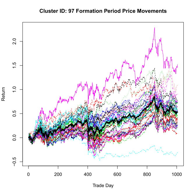
# Plot Equity Cluster Price Movement
CKret = (Kret + 1)
CKret = apply(CKret, 1, cumprod) – 1
matplot(CKret, type = ‘l’, xlab = ‘Trade Day’, ylab = ‘Return’,
main = paste(‘Cluster ID:’, Kid %>% as.character(), ‘Formation Period Price Movements’))
lines( ((apply(Kret, 2, mean) + 1) %>% cumprod()) – 1,
type = ‘l’, lwd = 3)
rm(CKret)
kandidates = 0 # Index for the number of cointegrateable members
# if(dev.cur() > 1){dev.off()} # Clear plots
if(exists(‘trade.cluster’) == TRUE){rm(trade.cluster)}
for(n in 1:length(Kid.e)){
# Create cumml return vector for equity (n)
sReturn = Kret[row.names(Kret) == Kid.e[n], ] + 1
sReturn = (sReturn %>% cumprod()) – 1
# Create cumml return vector for portfolio of all other members
pReturn = Kret[row.names(Kret) != Kid.e[n], ]
pReturn = apply(pReturn, 2, mean) + 1
pReturn = (pReturn %>% cumprod()) – 1
# mReturn = rbind(pReturn, sReturn)
# plot(mReturn[which.max(mReturn[,dim(mReturn)[2]]), ], type = ‘l’)
# lines(mReturn[which.min(mReturn[,dim(mReturn)[2]]), ], type = ‘S’)
# Regress equity returns on portfolio returns & test stationarity
lfit = lm(sReturn ~ pReturn) # Linear Regression
options(warn = -1)
lfit.adf = adf.test(lfit$residuals, k = 1) # Augmented Dickey-Fuller test on residuals
options(warn = 0)
if(lfit.adf$p.value <= param.dfp ){
# Itterate Index Counts
candidates = candidates + 1
kandidates = kandidates + 1
print(n %>% as.character())
# Back-teting in Current Period %%%%%%%%%%%%%%%%%%%%%%%%%%%%
# … Assumptions ….
# 1) No transaction costs
# 2) Trade is opened two-days after divergence
# 3) Trade is closed one-day after convergence
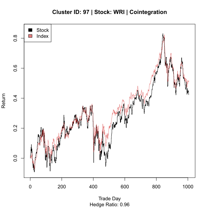
# Plotting Parameters
mainLab = paste(‘Cluster ID:’, Kid %>% as.character(), ‘|’,
‘Stock:’, Kid.e[n])
yLims = c(c(sReturn,pReturn) %>% min(),
c(sReturn,pReturn) %>% max())
hedgeRatio = lfit$coefficients[2] # Hedge-ration based on linear fit
dReturns = sReturn – pReturn*hedgeRatio # Difference-returns of hedged trade
plot(sReturn, type = ‘S’, ylim = yLims, main = paste(mainLab, ‘| Cointegration’),
xlab = ‘Trade Day’, ylab = ‘Return’,
sub = paste(‘Hedge Ratio:’, hedgeRatio %>% round(digits = 2) %>% as.character()) )
lines(pReturn*hedgeRatio, col = alpha(‘red3’, .5))
legend(“topleft”, inset=0, c(“Stock”,”Index”),
fill = c(‘black’, alpha(‘red3’, .5)), horiz=FALSE)
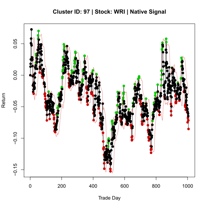
thld.buy = rollapply(dReturns, param.rld, align = ‘right’, mean) + param.sdm*rollapply(dReturns, param.rld, align = ‘right’, sd)
thld.sell = rollapply(dReturns, param.rld, align = ‘right’, mean) – param.sdm*rollapply(dReturns, param.rld, align = ‘right’, sd)
signal = rep(0, length(thld.buy))
dReturns.comp = dReturns[param.rld:length(dReturns)]
signal[dReturns.comp >= thld.buy] = 1
signal[dReturns.comp <= thld.sell] = -1
rm(dReturns.comp)
# plot(signal, type = ‘S’)
# Align moving …
signal = c(rep(0, (param.rld – 1)), signal)
thld.buy = c(rep(0, (param.rld – 1)), thld.buy)
thld.sell = c(rep(0, (param.rld – 1)), thld.sell)
signal.col = rep(‘black’, length(dReturns))
signal.col[signal == 1] = ‘green3’
signal.col[signal == -1] = ‘red3’
plot(dReturns, type = ‘S’, main = paste(mainLab, ‘| Native Signal’), xlab = ‘Trade Day’, ylab = ‘Return’)
points(dReturns, col = signal.col, pch = 19)
lines(thld.buy, col = alpha(‘red3’, .5))
lines(thld.sell, col = alpha(‘red3’, .5))
# Signal Openning Smoothing
signal.aug = c(0,0,signal[1:(length(signal)-2)])
signal.aug[which(signal == 0)] = 0
aug.rle = rle(signal.aug)
aug.rle$values[aug.rle$values != 0 & aug.rle$lengths == 1] = 0
signal.aug = sapply(c(1:length(aug.rle$lengths)), function(x) rep(aug.rle$values[x], aug.rle$lengths[x])) %>% unlist()
# Signal Closing Delay
aug.rle = rle(signal.aug)
for(x in 2:length(aug.rle$lengths)){
if(aug.rle$values[x-1] != 0){
aug.rle$lengths[x-1] = aug.rle$lengths[x-1] + 1
aug.rle$lengths[x] = aug.rle$lengths[x] – 1
}
}
signal.aug = sapply(c(1:length(aug.rle$lengths)), function(x) rep(aug.rle$values[x], aug.rle$lengths[x])) %>% unlist()
# Plot Comparison between Origina & Augmented Trade Signals
plot(signal, type = ‘S’, main = paste(mainLab, ‘| Signal Augmentation’), xlab = ‘Trade Day’)
lines(signal.aug*.5, type = ‘S’, col = alpha(‘red3’, .8), lwd = 2)
# Plot Augmented Signal on back-testing returns
signal.aug.col = rep(‘black’, length(signal.aug))
signal.aug.col[signal.aug == 1] = ‘green3’
signal.aug.col[signal.aug == -1] = ‘red3’
plot(dReturns, type = ‘S’, main = paste(mainLab, ‘| Augmented Signal’))
lines(thld.buy, lwd = 2, col = alpha(‘red’, .5))
lines(thld.sell, lwd = 2, col = alpha(‘red’, .5))
points(dReturns, col = signal.aug.col, pch = 19)
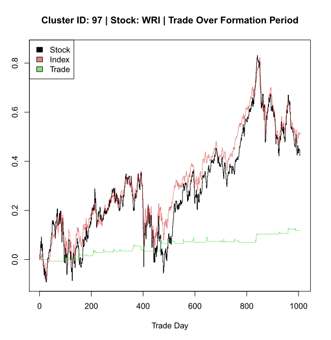
sret = Kret[Kid.e[n], ] # Daily equity returns
pret = Kret[Kid.e[-n], ] # Daily portfolio returns, hedged
pret = apply(pret, 2, mean)
dret = (sret – pret*hedgeRatio)*signal.aug; rm(sret, pret) # daily trade difference
dret = ((1 + dret) %>% cumprod()) – 1 # cummulative
plot(sReturn, type = ‘S’, ylim = yLims, main = paste(mainLab, ‘| Trade Over Formation Period’), xlab = ‘Trade Day’, ylab = ‘Trade Day’)
lines(pReturn*hedgeRatio, col = alpha(‘red3’, .5))
lines(dret, col = alpha(‘green3’, .5))
legend(“topleft”, inset=0, c(“Stock”,”Index”,”Trade”),
fill = c(‘black’, alpha(‘red3’, .5), alpha(‘green3’, .5)), horiz=FALSE)
# Record Pairs-trading Parameters
temp = data.frame(clusterSizes$ClustId[j], n, Kid.e[n], hedgeRatio, lfit.adf$p.value, row.names = NULL)
names(temp) = c(‘CluserId’, ‘MemberId’, ‘MemberName’, ‘HedgeRatio’, ‘ADF_pValue’)
if(exists(‘trade.cluster’) == FALSE){
trade.cluster = temp
}else{
trade.cluster = rbind(trade.cluster, temp)
}
}
}
# Back-test cointegrated pairs using next 6-months of returns
if(kandidates > 0){
# Get Price Data for Cluster & SP500 %%%%%%%%%%%%%%%%%%%%%%%%%%%%
testDate = trainDate[2]
testDate[2] = testDate[1] %m+% months(param.testLength)
# Get Market Index Data For Reference
getSymbols(Symbols = ‘SPY’, from = testDate[1], to = testDate[2]) # SPDR S&P 500 ETF (SPY), S&P500 Data from Yahoo is corrupted at the moment
SPY$SPY.ret = SPY$SPY.Adjusted %>% log() %>% diff(); SPY$SPY.ret[1] = 0 # Daily cc-returns
SPY$SPY.cret = ((SPY$SPY.ret + 1) %>% cumprod()) – 1 # Cummulative cc-returns
SPY.test = SPY; rm(SPY)
# Get Price Data for Cluster Members
test = BatchGetSymbols(tickers = Kid.e, first.date = testDate[1], last.date = testDate[2])
# Create matrix of Member Daily Returns %%%%%%%%%%%%%%%%%%%%%%%%%%%%
test.Pbardata = lapply(unique(test$df.tickers$ticker), function(x){return(test$df.tickers[test$df.tickers$ticker == x, ])})
names(test.Pbardata) = unique(test$df.tickers$ticker)
test.Pbardata.pradj = lapply(test.Pbardata, function(x){return(x$price.adjusted)}) # List of Adjusted Close Prices
test.Pbardata.retn = lapply(test.Pbardata.pradj, function(x){x %>% log() %>% diff()}) # List of daily-returns
rm(test.Pbardata.pradj, test.Pbardata)
# Clean any bad-data
retn.cnt = sapply(test.Pbardata.retn, length) %>% unlist() %>% plyr::count()
retn.cnt = retn.cnt$x[which.max(retn.cnt$freq)]
test.Pbardata.retn = lapply(test.Pbardata.retn, function(x) {if(length(x) == retn.cnt){return(x)}}) %>% compact()
test.retn = do.call(cbind, test.Pbardata.retn) %>% t()
test.retn = cbind(rep(0, dim(test.retn)[1]), test.retn)
# Back-test over forward-looking testing period %%%%%%%%%%%%%%%%%%%%%%%%%%%%
# if(dev.cur() > 1){dev.off()}
for(n in 1:kandidates){
# Plotting Header
mainLab = paste(‘Cluster ID:’, trade.cluster$CluserId[n] %>% as.character(), ‘|’,
‘Stock:’, trade.cluster$MemberName[n])
# Create cumml return vector for equity (n)
sReturn = test.retn[row.names(test.retn) == trade.cluster$MemberName[n], ] + 1
sReturn = (sReturn %>% cumprod()) – 1
# Create cumml return vector for portfolio of all other members
pReturn = test.retn[row.names(test.retn) != trade.cluster$MemberName[n], ]
pReturn = apply(pReturn, 2, mean) + 1
pReturn = (pReturn %>% cumprod()) – 1
yLims = c(c(sReturn, pReturn) %>% min(),
c(sReturn, pReturn) %>% max())
plot(sReturn, type = ‘S’, ylim = yLims, main = paste(mainLab,’| Cointegration over Test Period’))
lines(pReturn*trade.cluster$HedgeRatio[n], type = ‘S’, col = alpha(‘red3’, .5))
# Difference-returns of hedged trade
dReturns = sReturn – pReturn*trade.cluster$HedgeRatio[n]
thld.buy = rollapply(dReturns, param.rld, align = ‘right’, mean) + param.sdm*rollapply(dReturns, param.rld, align = ‘right’, sd)
thld.sell = rollapply(dReturns, param.rld, align = ‘right’, mean) – param.sdm*rollapply(dReturns, param.rld, align = ‘right’, sd)
signal = rep(0, length(thld.buy))
dReturns.comp = dReturns[param.rld:length(dReturns)]
signal[dReturns.comp >= thld.buy] = 1
signal[dReturns.comp <= thld.sell] = -1
rm(dReturns.comp)
# Align moving …
signal = c(rep(0, (param.rld – 1)), signal)
thld.buy = c(rep(0, (param.rld – 1)), thld.buy)
thld.sell = c(rep(0, (param.rld – 1)), thld.sell)
signal.col = rep(‘black’, length(dReturns))
signal.col[signal == 1] = ‘green3’
signal.col[signal == -1] = ‘red3’
plot(dReturns, type = ‘S’, main = paste(mainLab, ‘| Test Period Native Signal’))
points(dReturns, col = signal.col, pch = 19)
lines(thld.buy, col = alpha(‘red3’, .5))
lines(thld.sell, col = alpha(‘red3’, .5))
# Signal Openning Smoothing
signal.aug = c(0,0,signal[1:(length(signal)-2)])
signal.aug[which(signal == 0)] = 0
aug.rle = rle(signal.aug)
aug.rle$values[aug.rle$values != 0 & aug.rle$lengths == 1] = 0
signal.aug = sapply(c(1:length(aug.rle$lengths)), function(x) rep(aug.rle$values[x], aug.rle$lengths[x])) %>% unlist()
# Signal Closing Delay
aug.rle = rle(signal.aug)
for(x in 2:length(aug.rle$lengths)){
if(aug.rle$values[x-1] != 0){
aug.rle$lengths[x-1] = aug.rle$lengths[x-1] + 1
aug.rle$lengths[x] = aug.rle$lengths[x] – 1
}
}
signal.aug = sapply(c(1:length(aug.rle$lengths)), function(x) rep(aug.rle$values[x], aug.rle$lengths[x])) %>% unlist()
# Plot Comparison between Origina & Augmented Trade Signals
plot(signal, type = ‘S’, main = paste(mainLab, ‘| Test Period Signal Augmentation’))
lines(signal.aug*.5, type = ‘S’, col = alpha(‘red3’, .8), lwd = 2)
# Plot Augmented Signal on back-testing returns
signal.aug.col = rep(‘black’, length(signal.aug))
signal.aug.col[signal.aug == 1] = ‘green3’
signal.aug.col[signal.aug == -1] = ‘red3’
plot(dReturns, type = ‘S’, main = paste(mainLab, ‘| Test Period Augmented Signal’))
lines(thld.buy, lwd = 2, col = alpha(‘red’, .5))
lines(thld.sell, lwd = 2, col = alpha(‘red’, .5))
points(dReturns, col = signal.aug.col, pch = 19)
sret = test.retn[row.names(test.retn) == trade.cluster$MemberName[n], ] # Daily Returns for Equity
pret = test.retn[row.names(test.retn) != trade.cluster$MemberName[n], ] # Daily Returns for Portfolio
pret = apply(pret, 2, mean); pret = pret*trade.cluster$HedgeRatio[n]
tReturn = (sret – pret)
rm(sret, pret)
tReturn = tReturn * signal.aug
tReturn = ((tReturn + 1) %>% cumprod()) – 1
plot(sReturn, type = ‘S’, ylim = yLims, main = paste(mainLab, ‘| Trade Over Test Period’))
lines(pReturn*trade.cluster$HedgeRatio[n], type = ‘S’, col = alpha(‘red3’, .5))
lines(tReturn, type = ‘S’, col = alpha(‘green3’, .5))
}
}
}
dev.off()
